
By Dr. Charles Kironji Gatebe, NASA Scientist for GLOBE Student Research Campaign on Climate
The next morning, we arrive at the sampling site and proceed to extract the filters on which atmospheric particle (or aerosol) samples have been collected by the Streaker sampler shown in Figure 5, and to replace them with new filters. This filter exchange operation has to be performed with great care, as any mistakes, however small, can be costly and could lead to loss of data collected over a whole month’s period, or cause damage to the new filters we are about to load. This can be a difficult thing to do, given that we are working outside, sometimes in extreme weather conditions such as blizzards with strong winds in excess of 15 m/s, accompanied by snow and severe cold, coupled with the fact that our bodies still feel fatigued from the previous day’s steep climb and long walk. Nevertheless, we have to manage all these challenges with focused determination to accomplish our mission, which is one of the characteristics of a good scientist.
Our sampling station consists of a Streaker sampler (manufactured by PIXE International Corporation, Tallahassee, Florida, USA), a pump system, a battery, and a solar panel. The Streaker operates from a 12-volt battery with low power consumption, which allows us to run the instrument in the field for an extended period of time without access to electricity. The station is painted green to try to match the surrounding environment and, hence, reduce visual impacts to wildlife. The Streaker is a time-sequenced air-particulate sampler designed to sample particles in the air in two size groups: (i) fine – particles of size 2.5 microns and less, which is about 100 times thinner than a human hair, and (ii) coarse – particles of size 2.5–10 microns. With a flow rate of one liter per minute, air enters the inlet non-moving impaction stage (marked “A” in Figure 5b) onto a rotating impaction stage (“B”) and exits via a rotating filter stage (“C”), which retains most of the smaller particles. Note that stage “A” removes particles from the airstream larger than 10 microns and allows coarse and fine particles to pass through, and stage “B” collects coarse particles and allows fine particles to pass through to stage “C”, where they are deposited. Figures 6a and 6b show the two filters used with the Streaker. The Mylar filter (Fig. 6a; see also Fig. 5: stage filter “A”) looks like a plastic food wrap, but less sticky, and Fig. 6b, (see also Fig 5: stage “B”) is a Nuclepore filter with pore sizes of about 0.4 microns. If you would hold up these two particle filters to a light bulb, you would more easily see light through the Mylar than through the Nuclepore filter.
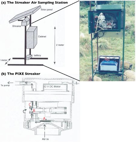
Figure 5a: Sampling Station, which consists of a Streaker sampler, a pump system, a solar panel, and 12-volts battery. Shown in the picture is a real pump system that is housed in a green-coated metal cabinet, while the battery is housed in a plastic case to protect it from extreme cold weather conditions. The height of the Streaker sampler is about 2 m above the ground. In Fig. 5b, as air enters and exits the Streaker sampler, particles in the airstream are deposited on either stage A, B or C. Larger particles are removed from the airstream at A, medium particles at B, and smaller particles at C.
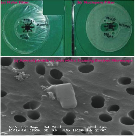
Figure 6: Special filters (a and b) that are used for particulate sampling, while (c) shows aerosols particles collected on a Nucleopore filter, magnified tens of thousands of times by an electron microscope.
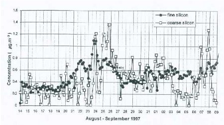
Figure 7a: Time series of 4-hourly concentrations of silicon obtained from the analysis of coarse and fine filters.
The two particle filters can be analyzed in a laboratory to determine chemical composition of the collected aerosol samples, using ion-beam methods such as X-rays, as shown in the Fig. 6c example. This allows a direct link to be established between particulate pollution measured at the mountain site with long-range transport of particles at high altitudes in the atmosphere. If we were to look at a time series of the concentrations of different chemical elements plotted on the same graph from measurements taken several times a day (our data has a time interval of about 4 hours over a period of 28 days), we can see changes (increase or decrease) in the concentrations of these elements, following changes in the local daily wind. However, when a moving time averaging of 36 hours is performed, it removes diurnal changes caused by upslope–downslope winds, and reveals variations associated with wind patterns caused by large scale weather systems, such as pressure differences over large areas, or storm systems such as hurricanes or cyclones. From past studies, it has been found that local circulation systems affect aerosol concentration several times a day as demonstrated in Figure 7a, while longer time-scale variations superimposed on the diurnal variations can be observed in the smoothed time series curves, as shown in Figure 7b. It is generally assumed that fine particles are transported over longer distances than coarse particles, although there is evidence that dust from the Sahara desert, containing a large fraction of coarse-size particles, is transported across the Atlantic Ocean to the USA, the Carribean, and parts of South America within a few days. This assumption makes it easier to differentiate between changes in particulate chemical concentration associated with local sources and those associated with distant sources, and transported to the site by the free tropopheric air. This type of experiment is possible on a high mountain such as Mt. Kenya, which allows sampling in the free troposphere, especially at night when the winds are predominantly blowing downslope and far removed from major pollution sources, and therefore represent pollution from distant places.
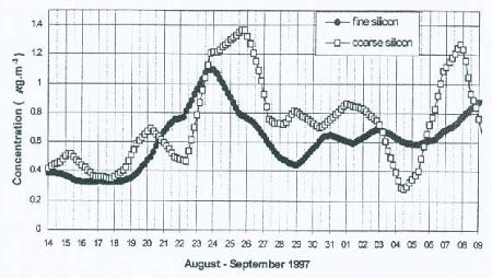
Figure 7b: 36-hour moving average of the 4 hourly data shown in Figure 7a.
After we change the samples, we decide to go down the mountain using a trail that takes us through the northern side of the mountain and through a permanent monitoring site, shown in Figure 8, run by the Kenya Meteorological Department under the World Meteorological Organization (WMO), Global Atmospheric Watch Program (GAW). This station monitors greenhouse gases such as carbon dioxide and methane, and basic meteorological parameters such as pressure, humidity, temperature, wind speed, wind direction, and radiation on a continuous basis. For more information on the GAW station visit their web site at: gaw.empa.ch/gawsis/reports.asp. The WMO data collection site, like many others located elsewhere in the world, provides valuable data that students from all over the world can download for free and use in climate related research. Try examining some of the data yourself. Look for changes in chemical concentrations with time, and see if you can establish any correlation with weather parameters such as wind speed and direction, humidity, radiation, etc., or try to identify sources of pollution in your area such as industries or factories, motor vehicles, and fires.
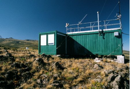
Figure 8: Mt Kenya GAW Station established in 1999. Picture from http://gaw.empa.ch/gawsis/reports.asp?StationID=57.
The trek down the mountain is much easier, especially if your knees are strong, and it takes much less time to get to the base station. I will let you enjoy the rest of the walk from the GAW site to the base station, and hope that this blog inspires many of you to think of a climate related research and to participate in the GLOBE’s Student Climate Research Campaign. In future, we will discuss NASA satellites that can be used for monitoring air pollution.