by Dr. Peggy LeMone, NCAR Scientist, former GLOBE Chief Scientist and President-Elect of the American Meteorological Society
Have you ever wondered how people test climate models? We used to have a joke that climate modelers had the best job security – because no one would know if their models were right or not until after they died.
Actually, climate models are being tested all the time. How is this done? A variety of ways. Here, I’m going to discuss how climate models are tested, based on some things I learned recently at a symposium on Paleoclimates, sponsored by the Western Interior Paleontological Society (WIPS). The figures are from one of the keynote addresses, by Dr. Caspar Ammann of NCAR.
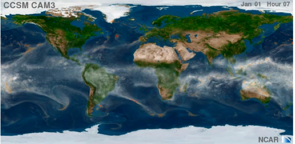
First, climate models are tested by seeing if they can replicate the current climate. Figure 1 shows one such simulation. The image looks a lot like a satellite view of the weather on Earth – with the long strings of white looking like warm and cold fronts. Also, notice the concentration of water vapor near the Equator. This is the Inter Tropical Convergence Zone (ITCZ), where air comes together from the northern and southern hemispheres, and then rises. This is a “gut test” – the model results look right. If you follow this simulation through the year (and we did at the NCAR Visualization Lab), you can see the progress of the Indian monsoon, and the formation of a couple of tropical cyclones (though you need pretty high horizontal resolution for that). I should note that the simulation is for a “typical” year in today’s climate. That is – you won’t find a January 1 that looks exactly like this.

Figure 1. Total water vapor in a vertical column in the atmosphere. Areas with more water vapor look white, intense concentrations are orange. Courtesy James Hack, NCAR. (download at: http://www.vets.ucar.edu/vg/T341/index.shtml)
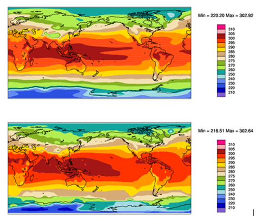
Climate models are designed to give us statistics about the weather, rather than specific real world weather events. For example, the climate model should be expected to do a reasonable job of reproducing the mean surface temperature over a season or over a year. Such a comparison is illustrated in Figure 2. The general temperature patterns are remarkably similar.

Figure 2. Surface air temperature. Top, from the Coupled Climate System Model, Version 3. Bottom, from observations. The relationship of colors to temperature is shown by the color bars to the right. Courtesy Caspar Ammann, NCAR.
Climate scientists also test parts of their models. To understand this, let’s describe a climate model. Like a weather model, the climate model solves equations for temperature, wind, water vapor, etc., on a three-dimensional grid of points. For example, take a grid point 3,000 m above Dakar, Senegal. Suppose the wind is out of the south, and the air is warmer to the south. The model would “predict” that the wind would carry in warmer air, to warm the temperature by a specific amount. Solar radiation, and longwave radiation (heat) from the ground and surrounding air layers would affect the temperature at this point, too. Adding all these effects at each point will give a new temperature. The same thing is done for wind, humidity, and whatever other variables the model is trying to predict.
Now imagine lots of these points – all over the Earth, and at heights from just above the surface to far up in the atmosphere. Obviously, we need a computer to make all these predictions. These predictions are made for specified time intervals, which vary with the grid spacing (and type of model). The first set of values on the grid leads to a second prediction. The second set of values on the grid leads to a third prediction, and so on. For weather forecast models, the calculations are repeated for a few calendar days. For climate prediction, the predictions can run for a thousand years. (Of course the computer run will take a much shorter time than 1,000 years – otherwise the forecast wouldn’t be very useful! To avoid confusion, scientists sometimes refer to “model time” (1,000 years) to contrast that with how long it took to run the model (much less)
We’d like these points to be as close together as possible, but the number of points is limited by the size and speed of computers, so the points are farther apart for climate models than for weather models.
Because of this, the effects of things like thunderstorms have to be estimated using what we call “parameterization schemes.” If a thunderstorm went through our point 3,000 m over Dakar, the model would allow for that by changing the temperature (and wind, and humidity, etc.).
Climate models have also to account for changes in the ocean, and changes in the land surface, including ice and vegetation and soil. The model will account for wet soil warming up the air more slowly than dry soil (but at the same time evaporation would transfer moisture from the soil into the atmosphere where it can later condense and release that stored heat), and solar radiation reflecting off an icy or snowy surface. The amount of detail on the surface can vary from model run to model run.
And this leads to another way the models are tested – each of these parameterization schemes is tested. Sometimes, observations are used. These can be data routinely gathered using satellites, or data gathered in a field campaign focused on a specific phenomenon – like thunderstorms, or like stratus clouds to the west of continents.
Anytime observations are used, the model is tested for the “current” climate state, or its variability. But how can we be sure that the same model also might do a reasonable job for future climates when we expect things to be different?
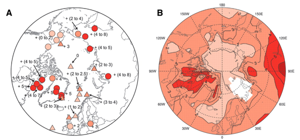
For this, one option climate scientists have is to simulate past climates. Because we have some information about past climates, we can see how well models reproduce them. We all learn that our climate has changed over the age of the Earth. For example, North America and Europe have had repeated glaciations during the last couple million years. Figure 3 shows an example of one such simulation, with temperatures compared to the climate simulation.

Figure 3. Comparison of a climate simulation to temperature estimates, for the last interglacial, about 130,000 years ago. On the left side are real world proxy-based reconstructions of maximum summer temperature (circles are land records, triangles are marine records), on the right side is a model simulation that was done applying information about the Earths orbital configuration of that time. (Adapted from Figure 2, from Otto-Bliesner, B.L., S.J. Marshall, J.T. Overpeck, G.H. Miller A. Hu, and CAPE Last Interglacial Project Members, 2006: Simulating Arctic climate warmth and icefield retreat in the last Intergaciation Science, New Series, v. 311, No 5768, ;1751-1753.)
How do we know how the temperatures changed during geologic time? We use other evidence (referred to as “proxies.”) Much of the dicussion at thew WIPS symposium was about this topic. Here are just a few ways:
1. Measuring the ratio of “heavy oxygen” (Oxygen-18, or oxygen with an atomic weight of 18) to light oxygen (the “normal” oxygen isotope, with an atomic weight of 16). Since “lighter” water molecules evaporate more readily at cooler temperatures, more of it rises into the atmosphere to form precipitation, which is stored in the ice sheets during ice ages. Thus more “light” oxygen in ice means cooler temperatures.
2. Counting the teeth on the boundary of leaves. The number of teeth is related to temperature.
3. Determining from fossil leaves and pollen what type of vegetation lived in a given area. If these are for the same (or similar species) that live today, this provides information about the climate under which the plant grew.
4. From the temperature range of the nearest living relative of fossil animals.
5. Looking at the fraction of Oxygen-18 in foraminifera, tiny (usually less than 1 mm across) little animals with shells that lived primarily in the oceans.
6. Looking at the type of insect damage in plants provides clues about how tropical the climate was.
7. Structure of a specific type of molecule (tetraethers) is a strong function of temperature at the time of its formation.
8. And many, many more…
Similarly, fossil evidence provides clues about how rainy it was. For example, the minerals deposited in channels formed by roots vary with how well-drained the soils were, and hence how dry the soil was. And fossils of lush, tropical plants are associated with rainy climates.
Simulations of these ancient climates aren’t always consistent with the data – but scientists are finding that comparisons with paleoclimates can lead to both improvements in climate models – and sometimes, a refinement in the observations!
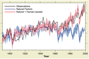
Given that, I’m going to show you my favorite simulation, which puts modern day influences on climate in perspective.

Figure 4. Simulation of climate for the last century. Blue includes experiments where only natural forcing factors were affecting climate: volcanoes and solar output. The red/pink simulations also include the effects of changes in greenhouse gases and dust produced by humans. The black line is the observed temperature record. (dapted from Figure 2, of Meehl, G.A., W.M. Washington, C.M. Ammann, J.M. Arblaster, T.M.L. Wigley, and C. Tebaldi, 2004: Combinations of Natural and Anthropologic Forcings in Twentieth-Century Climate. J. Climate, 17, 3721–3727.)
From Figure 4, one obtains the current warming record only if the effects of greenhouse gases are included.
Climate scientists continue to test their models – and improve them. This is being done through improving the parameterizations, and, with time, running at higher resolution (smaller grid sizes). With these improvements, climate scientists should be able not only to improve projected global average statistics, but they should be able to look at future climates in different parts of the world. The Holy Grail (ultimate goal) of climate modeling then is if model can do both global trends and regional impacts in both mean but also in variability, including the information about changes in extreme events!
